 GOVERNMENT
OF INDIA
GOVERNMENT
OF INDIA
A Digital India Initiative
Please login using your email address as it is mandatory to access all the services of community.data.gov.in
GOVERNMENT
OF INDIA


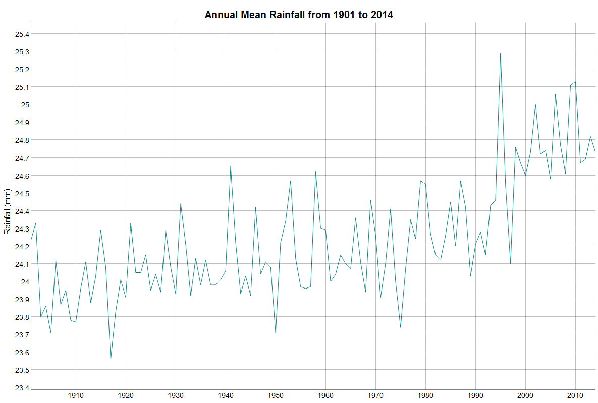
Our country (India) is diversified. A lot of variation can be seen from North to South and East to West. Top side of country is having a range of Mountains that starts from Jammu & Kashmir to Arunachal Pradesh; Middle part of country is having plains. Most of the south part of country is covered by sea. These parameters are responsible for the variation of climate that leads to cause of variations in rainfall that is why some parts of India are rich in rainfall and some parts of India are rain deficient.
In this blog, I am doing some analysis like forecasting of annual rainfall in India in coming years. For the experiment, I have taken data of Mean Annual Rainfall from www.data.gov.in. The data is having the information of mean annual rainfall from year 1901 to 2014. Take a look of data as shown below.
In this experiment I have taken the help of R programming that is now one of most demanded software in the field of data science and statistics. For the analysis, first column of the dataset is chosen to do analysis that is having annual mean rainfall information in mm unit.
Reading of Data:
In R, read.csv and read.table functions are available to read the datasets like csv/txt.
setwd("D:/")

d=read.csv("MEAN.csv")
head(d)
ANNUAL JAN.FEB MAR.MAY JUN.SEP OCT.DEC
1901 24.23 18.71 26.06 27.30 21.92
1902 24.33 19.70 26.44 27.18 21.49
1903 23.80 19.05 25.47 27.17 21.27
1904 23.86 18.66 25.84 26.83 21.42
1905 23.71 17.58 24.99 27.37 21.48
1906 24.12 18.37 25.93 27.15 22.08
tail(d)
ANNUAL JAN.FEB MAR.MAY JUN.SEP OCT.DEC
2009 25.11 20.72 26.86 27.89 22.58
2010 25.13 20.19 27.83 27.50 22.60
2011 24.67 19.54 26.38 27.54 22.71
2012 24.69 19.34 26.55 27.71 22.35
2013 24.82 19.98 26.85 27.46 22.50
2014 24.73 19.58 26.24 27.88 22.47
Head function is used to show the upper 6 rows of the datasets similarly tail function shows the lower 6 rows. MEAN.csv is the main file that is having information of mean annual rainfall, first column has annually information, second columns has information from Jan to Feb similarly others have according to their column names. From the head and tail functions, it is evident that datasets is having information from 1901 to 2014.
Time Series Conversion:
This part is convert your dataset in time series object that make easy to use R’s many functions to analyze the dataset. For this purpose we use ts function.
annual=d[,1]

head(annual)

[1] 24.23 24.33 23.80 23.86 23.71 24.12
a=ts(annual,start=1901,end=2014,frequency = 1)
a
Time Series:
Start = 1901
End = 2014
Frequency = 1
[1] 24.23 24.33 23.80 23.86 23.71 24.12 23.87 23.95 23.78 23.77 23.96 24.11 23.88 24.03 24.29
[16] 24.08 23.56 23.83 24.01 23.91 24.33 24.05 24.05 24.15 23.95 24.04 23.94 24.29 24.08 23.93
[31] 24.44 24.21 23.92 24.13 23.98 24.12 23.98 23.98 24.01 24.06 24.65 24.22 23.93 24.03 23.92
[46] 24.42 24.04 24.11 24.08 23.71 24.22 24.34 24.57 24.13 23.97 23.96 23.97 24.62 24.30 24.29
[61] 24.00 24.04 24.15 24.10 24.07 24.36 24.11 23.94 24.46 24.26 23.91 24.10 24.41 24.00 23.74
[76] 24.07 24.35 24.24 24.57 24.55 24.27 24.15 24.12 24.26 24.45 24.20 24.57 24.42 24.03 24.21
[91] 24.28 24.15 24.43 24.46 25.29 24.55 24.10 24.76 24.67 24.60 24.73 25.00 24.72 24.74 24.58
[106] 25.06 24.77 24.61 25.11 25.13 24.67 24.69 24.82 24.73
In ts function start is having the initial time, end is having the time of last record and frequency stands for the collection of data like yearly=1 or quarterly=4 or monthly=12.
We have store annual mean rainfall data in object which is a time series object.
Simple Time Series Plot:
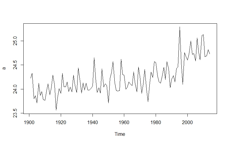
Now data is stored in a object, time series plot can be made by calling plot.ts function. It shows the annual mean rainfall from year 1901 to 2014.
Above image is obtained by using some advance packages in R. Simple plot can be obtained by using plot.ts. Code is shown below
plot.ts(a)
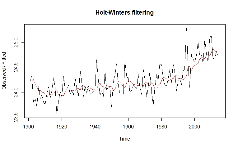
Simple Exponential Smoothing:
If the time series data has no seasonality then simple exponential smoothing can be used for short term forecasts. To do this step we are using HoltWinter function that is available in R. Set parameter beta and gamma false in HoltWinter function.
ha=HoltWinters(a,beta=F,gamma=F)
ha
Holt-Winters exponential smoothing without trend and without seasonal component.
Call:
HoltWinters(x = a, beta = F, gamma = F)
Smoothing parameters:
alpha: 0.2022571
beta : FALSE
gamma: FALSE
Coefficients:
[,1]
a 24.78922
alpha parameter is close to zero that indicates that forecasts are based on recent observations.
ha$fitted

Time Series:

Start = 1902

End = 2014

Frequency = 1

xhat    level

1902 24.23000 24.23000

1903 24.25023 24.25023

1904 24.15916 24.15916

1905 24.09866 24.09866

1906 24.02005 24.02005

1907 24.04026 24.04026

1908 24.00583 24.00583

1909 23.99454 23.99454

1910 23.95114 23.95114

1911 23.91451 23.91451

1912 23.92371 23.92371

1913 23.96139 23.96139

1914 23.94493 23.94493

1915 23.96213 23.96213
ha$SSE

[1] 6.43627
In above plot the black line shows the original time series and forecasts is red line.
ha$SSE : 6.43627 represents the accuracy of forecasts. SSE is sum of squared errors.
forecast.HoltWinters() function, takes predictive values fitted by using HoltWinters() function above. In the case of the rainfall time series, we stored the predictive model made using HoltWinters() in the variable “ha”. “h” defines as the number of further years we predict.
fha=forecast::forecast.HoltWinters(ha,h=10)

fha

Point Forecast    Lo 80    Hi 80    Lo 95    Hi 95

2015       24.78922 24.48362 25.09481 24.32184 25.25659

2016       24.78922 24.47743 25.10100 24.31238 25.26605

2017       24.78922 24.47136 25.10707 24.30310 25.27533

2018       24.78922 24.46541 25.11302 24.29400 25.28444

2019       24.78922 24.45956 25.11887 24.28505 25.29338

2020       24.78922 24.45382 25.12461 24.27627 25.30216

2021       24.78922 24.44817 25.13026 24.26763 25.31080

2022       24.78922 24.44261 25.13582 24.25913 25.31930

2023       24.78922 24.43715 25.14129 24.25077 25.32766

2024       24.78922 24.43176 25.14667 24.24254 25.33589
The forecast.HoltWinters function gives the predictive result of rainfall with 80% confidence interval and 95 percent of confidence interval. The forecast rainfall of 2020 is about 24.78922 with 80% prediction interval of (24.45382, 25.12461) and 90% prediction interval of (24.27627, 25.30216).
The plot of predicted values is shown below, that is obtained by suing plot.forecast function
forecast::plot.forecast(fha)
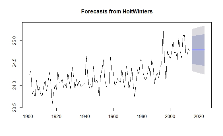
In the above graph, forecasts from 2015 to 2014 are shown in blue line 80% confidence interval is shown in light blue shade and 95% is shown in light grey shade region.
The ‘forecast errors’ are estimated as the observed values minus predicted values, for each time point. It is calculated only over original time series that is 1901 to 2014. Accuracy of predictive model is measured on the basis of SSE sum-of-squared-errors as shown above.